A notebook that models and analyses my personal finances for my first-year as an incoming University of Toronto, Faculty of Arts and Sciences student. Modeling on Pandas rather than a spreadsheet offers a few benefits on top of providing practice: it enables the application of some advanced statistical techniques not easily accessible in Excel, some advanced visualisation libraries, and so on. I have not utilised most of these features yet. I intend to extend this analysis further with a Monte Carlo simulation (as opposed to scenario based modeling) in the future, for instance.
Structure#
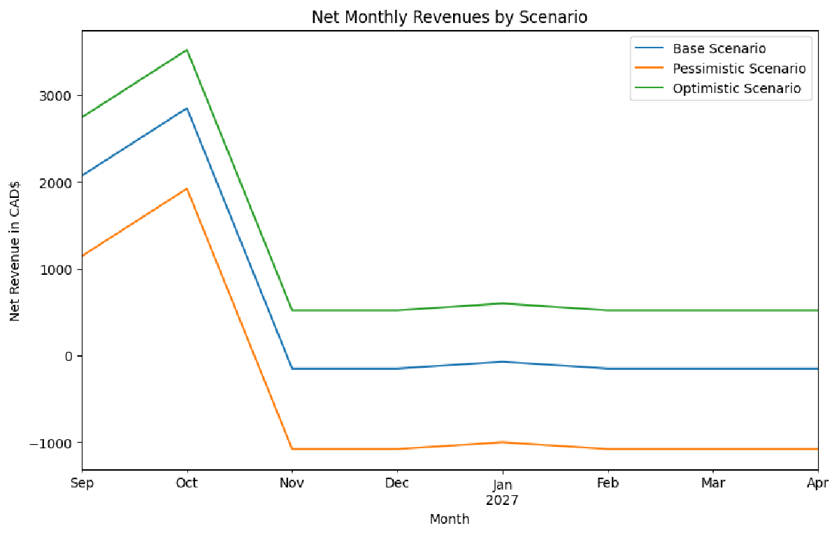
The notebook consists of cost, revenue, and net dataframes for base, pessimistic, and optimistic forecasts. In total, there are 9 such, ‘core’ dataframes. Costs are categorised largely according to the UofT Financial Planner. So too are revenues. I estimated OSAP and UTAPS grants and loans, and zeroed scholarships and family support for simplicities sake. My main revenues aside from these are: summer work, expressed as a starting balance added to my running balance in the net dataframes; part-time work, expressed as a constant revenue source. More on these later.
| Net | Running Balance | |
|---|---|---|
| Date | ||
| 2026-09-01 | 1144.0 | 6424.0 |
| 2026-10-01 | 1922.0 | 8346.0 |
| 2026-11-01 | -1078.0 | 7268.0 |
| 2026-12-01 | -1078.0 | 6190.0 |
| 2027-01-01 | -1000.0 | 5190.0 |
| 2027-02-01 | -1078.0 | 4112.0 |
| 2027-03-01 | -1078.0 | 3034.0 |
| 2027-04-01 | -1078.0 | 1956.0 |
After inputting all the relevant data and consolidating it into the three main models, I got to the core of my analysis: the use of aggregate metrics to analyse my forecast finances. I judged my finances by the following metrics:
- Final balance
- Minimum balance
- Maximum deficit
- Worst month
- Months negative
- Required buffer
| Final Balance | Minimum Balance | Max Deficit | Worst Month | Months Negative | Required Buffer | |
|---|---|---|---|---|---|---|
| Base | 13948.0 | 11927.0 | -151.0 | 2026-11-01 00:00:00 | 0 | 0 |
| Optimistic | 22140.0 | 15415.0 | 521.0 | 2026-11-01 00:00:00 | 0 | 0 |
| Pessimistic | 1956.0 | 1956.0 | -1078.0 | 2026-11-01 00:00:00 | 0 | 0 |
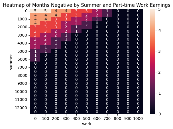
I also performed a sensitivity analysis on the two main variable revenues in my budget, part-time and summer work. The intention was to determine how much I could bend these variables and stay in the green. I visualised this in heatmaps, and a feasible frontier curve.
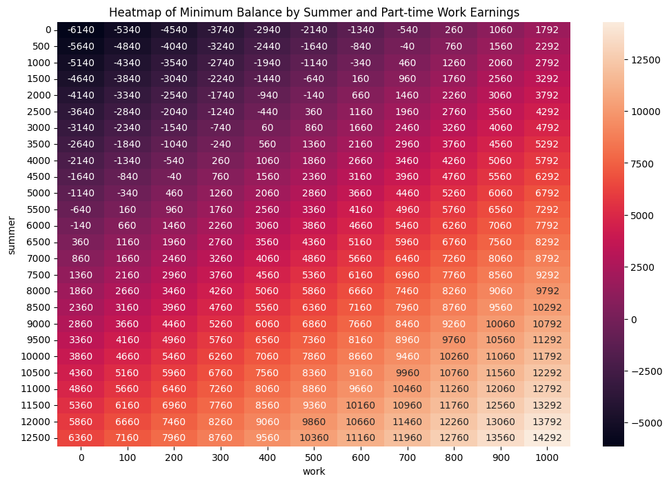
| Part-time Earnings | Summer Earnings | |
|---|---|---|
| 0 | 0 | 6500 |
| 1 | 100 | 5500 |
| 2 | 200 | 5000 |
| 3 | 300 | 4000 |
| 4 | 400 | 3000 |
| 5 | 500 | 2500 |
| 6 | 600 | 1500 |
| 7 | 700 | 1000 |
| 8 | 800 | 0 |
| 9 | 900 | 0 |
| 10 | 1000 | 0 |
The final aspect of this notebook was a residence cost, and then weighted, comparison. For the former, I manually input the costs for each residence available to me to see how they would mesh with my broader budget.
| Residence | Minimum Balance | Final Balance | Months Negative | Max Deficit | |
|---|---|---|---|---|---|
| 3 | New College | 2406 | 2406.0 | 0 | -3014.5 |
| 0 | Woodsworth | 1956 | 1956.0 | 0 | -1078.0 |
| 2 | Knox | 1475 | 1475.0 | 0 | -2183.0 |
| 6 | University College | 823 | 823.0 | 0 | -3806.0 |
| 1 | Chestnut | -2559 | -2560.0 | 4 | -3797.0 |
| 5 | Trinity | -5196 | -5197.0 | 4 | -6816.0 |
| 4 | Oak | -6962 | -6963.0 | 4 | -7699.0 |
After that, I had three LLMs (Claude 4.6, GPT-5.3, and Deepseek) rank the (first four) viable residences across a few similar categories. I got the following results:
| Cost | Room & Amenities | Community | Food | Location | |
|---|---|---|---|---|---|
| Woodsworth | 2 | 1 | 3 | 1 | 3 |
| Knox | 3 | 4 | 4 | 3 | 4 |
| UC | 4 | 3 | 1 | 4 | 1 |
| New College | 1 | 2 | 2 | 2 | 2 |
I weighted these categories according to my preferences, and then derived a ranking of residences.
| Weighted Ranking | |
|---|---|
| Woodsworth | 1.55 |
| New College | 1.95 |
| UC | 2.75 |
| Knox | 3.75 |
Analysis#
What lessons did I derive from this? I got a viable ranking of residences, which I have used in my StarRez application. OSAP and UTAPS applications ask the applicant for estimates regarding, among other things, their starting assets and work earnings expectations throughout the school year. I have a model that can inform the values I give when asked for such details. Not to mention that I have an idea of how hard I’ll need to actually work, this summer and the school year, in order to stay afloat, which is extremely useful. I also have a nice budget template, something I can refine based on my actual data even better in my second year.
Generally, my finances are viable so long as I earn either $1000 per month during the school year, save up $6500 this summer, or (in the middle) save $2500 and earn $500/month during the school year. This is all according to my pessimistic cost forecasts, so this is a worst case analysis.
It does, however, use OSAP and UTAPS estimates that are not guaranteed. I will have to update these with actual figures once I’ve applied. Moreover, it treats OSAP loans as if they were revenue - loans are liabilities.